New release R20230622
More solvers
More solvers
No more kittens
Save your F5
The first cut is not the deepest
Alternative to Google groups
From hard to a one-liner
Common mistakes and misunderstandings in semidefinite programming
Support for MathWorks coneprog
Not everyhing was better in the past
A whole lotta stuff
Various small improvements
Various small improvements
Be careful with unnecessary symbolic overhead
Various small improvements
Revised MISDP solvers
Minor fixes and improvements
Minor fixes and improvements
Minor fixes and improvements
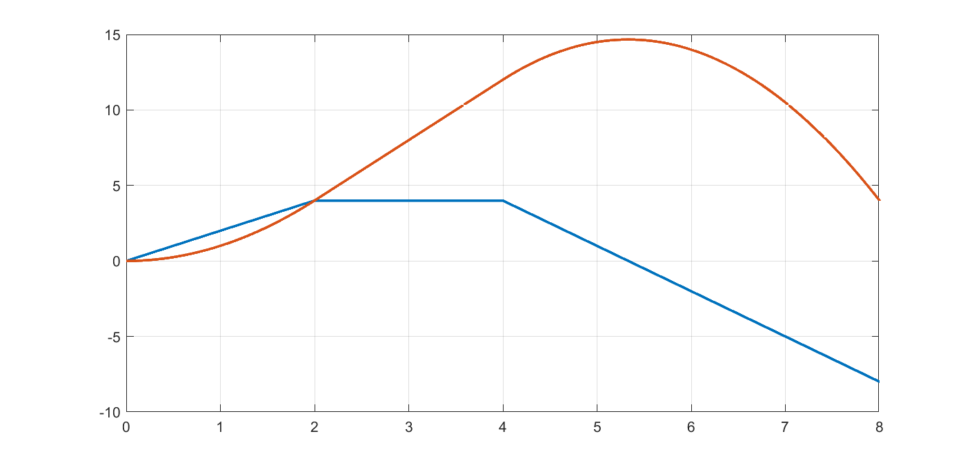
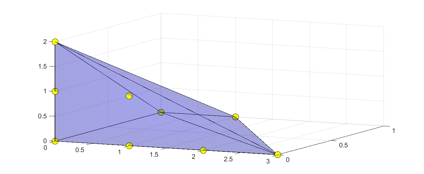
Working with polynomials, function values, derivatives, integrals and their properties
Minor fixes and improvements
Minor fixes and improvements
Important patch
Untangle that messy expression
Removed bug crashing bonmin and ipopt
Performance fix and extended interp1
Improvements in bmibnb, interp1 and sdisplay
There is more than one way to skin a cat
Some more fixes…
Update for cplex bug
New solvers and minor patches
Both patches and new features
It’s been a while…
MATLAB no longer required! Recommended though.
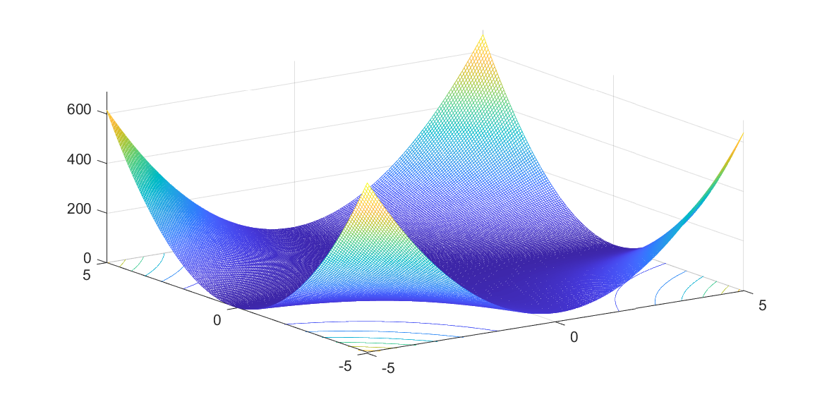
Hard? Let’s try anyway.
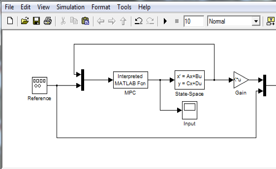
Using YALMIP objects and code in Simulink models, easy or fast, your choice.
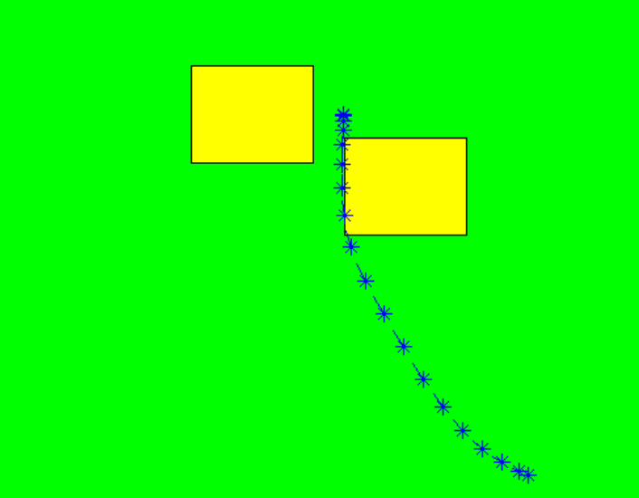
A common application of integer programming is the unit commitment problem in power generation, i.e., scheduling of set of power plants in order to meet a cu...
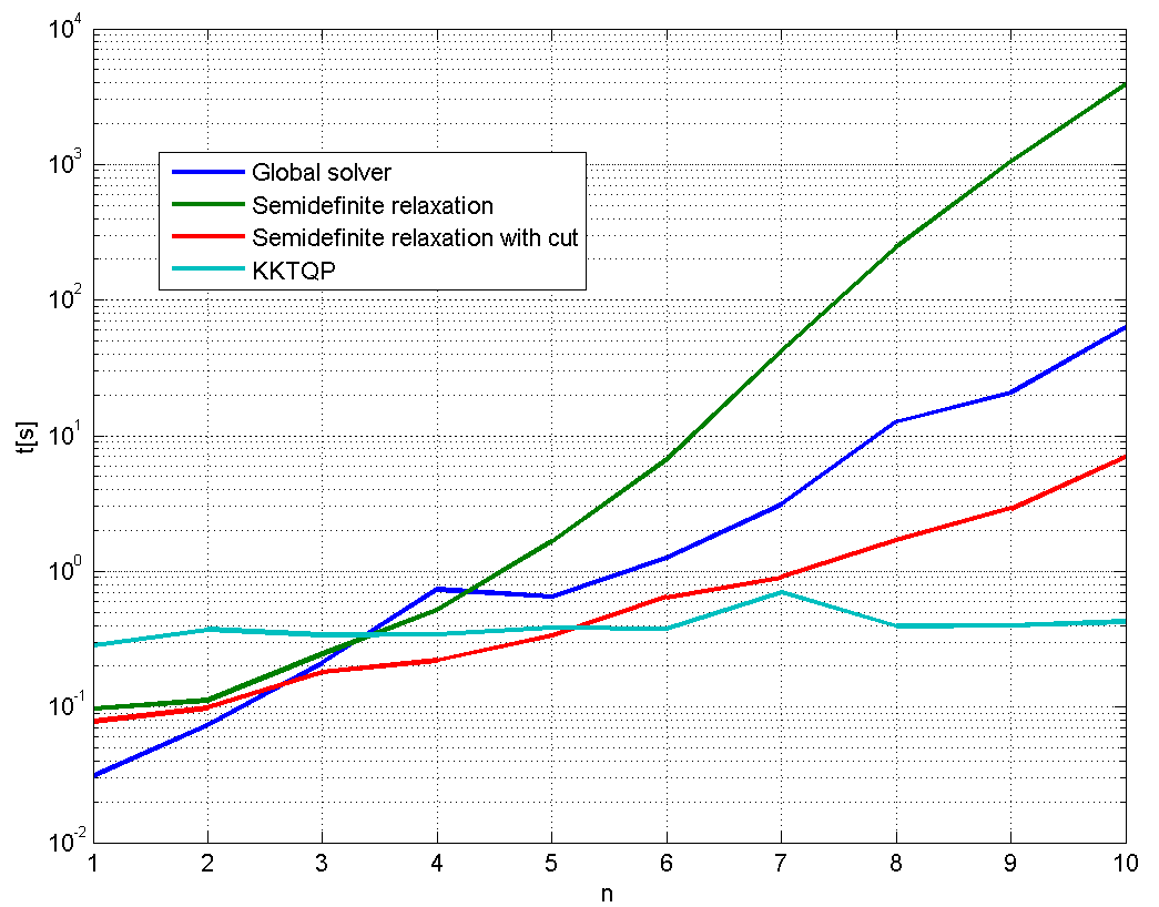
Common question: how can I solve a nonconvex QP using SeDuMi? Weird question, but interesting answer.
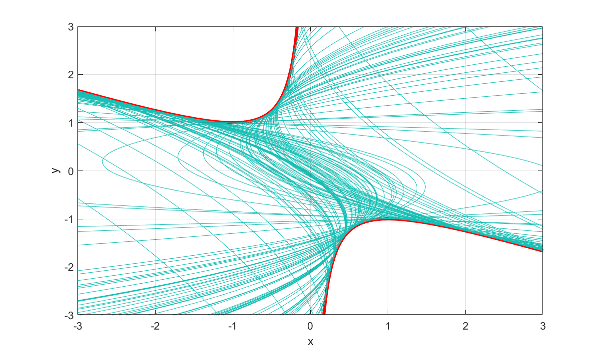
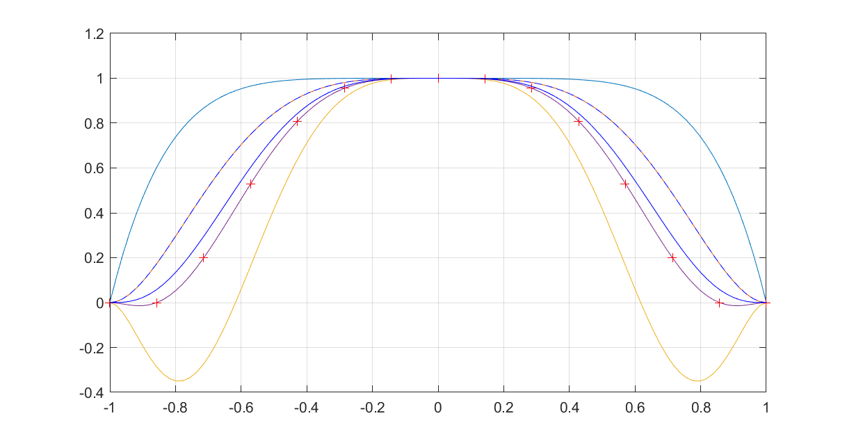
A question on the YALMIP forum essentially boiled down to how can I generate sum-of-squares solutions which really are feasible, i.e. true certificates?
Files and exercise material from the YALMIP work-shop at the Swedish control conference 2010
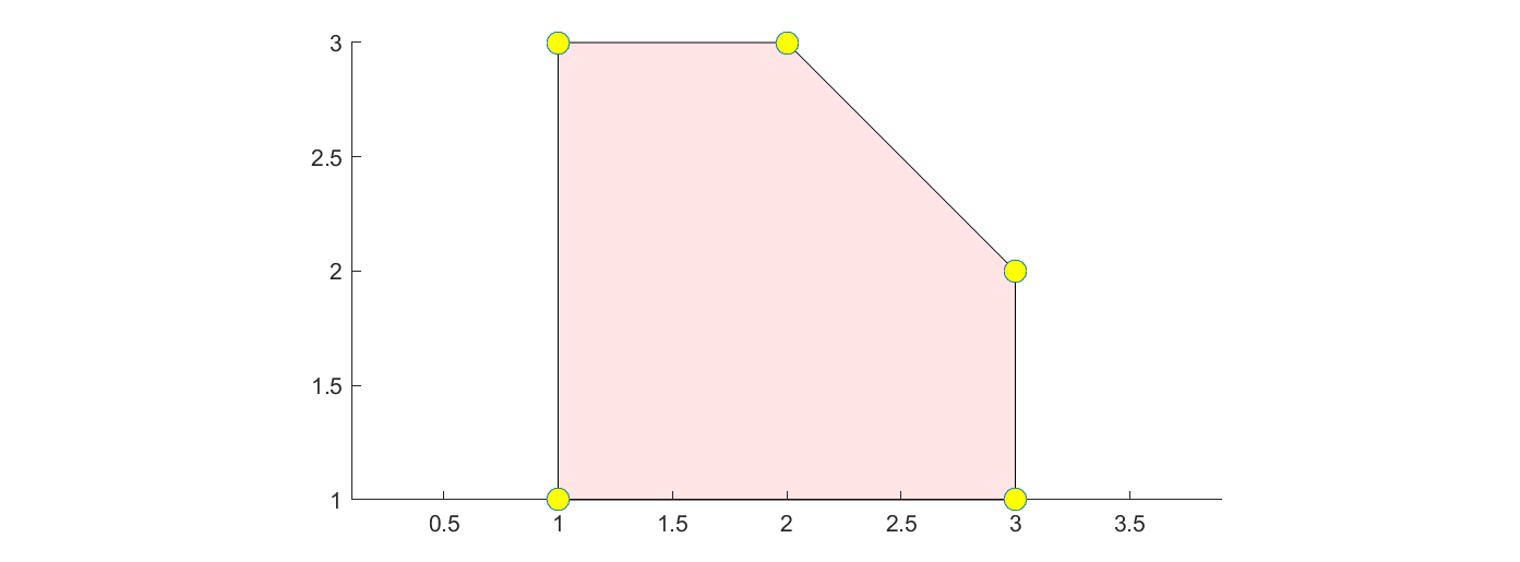
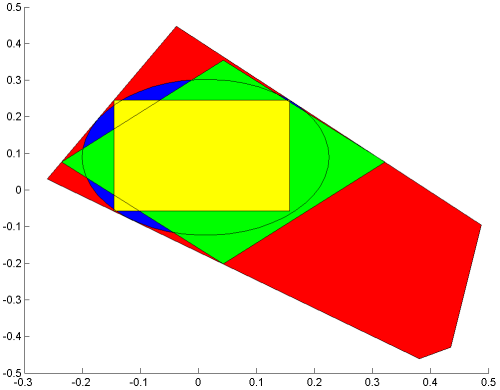
Ever wondered how to compute the L1 Chebyshev ball?
Added a sum-of-squares example focusing on pre- and post-processing capabilities.